How to Use the Weighted Average Formula in Excel – InstantFollowerz

When to use a weighted average

Use a weighted average when values ​​have different importance. But what exactly does that mean?

Here’s an example. Let’s say I want to buy a new home, but I’m not sure what the average market value is in my neighborhood. My budget is $350,000, so I’m looking at prices on five different houses:

• $1,000,000
• 800,000 dollars
• $400,000
• 300,000 dollars
• $250,000

If I use the simple average formula, I get $550,000, which is out of my price range. problem? My average is wrong. That’s because I didn’t take into account how many homes are selling for each price. Here’s the list again, but with the number of houses selling for that price in parentheses.

• $1,000,000 (1)
• $800,000 (2)
• $400,000 (10)
• $300,000 (25)
• $250,000 (15)

Using the weighted average formula allows me to take into account that only one home sells for a million dollars, while there are 25 times as many homes priced at $300,000. Using the weighted average formula, I get an average of $336,792, which is right in my wheelhouse.

It’s like magic, isn’t it? Here’s how it works.

How to calculate a weighted average in Excel

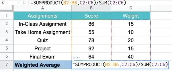
To calculate a weighted average in Excel, use the SUMPRODUCT and SUM functions in the following formula:

=SUMPRODUCT(X:X,X:X)/SUM(X:X)

This formula works by multiplying each value by a weight and combining the values. Then divide the SUM OF THE PRODUCT by the sum of the weights for your weighted average.

Still confused? Let’s move on to the steps in the next section.

Using SUMPRODUCT to calculate a weighted average in Excel

Here are my steps for using SUMPRODUCT.

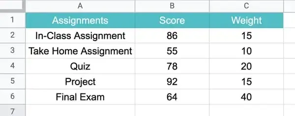
1. I enter my data into a table and then add a column containing the weight for each data point.

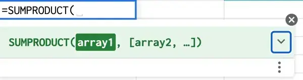
2. Then I type =SUMPRODUCT to run the formula and enter the values.

3. Finally, I click enter to get my results.

Here’s what’s going on under the hood.

First, the equation multiplies each score by its weight:

• 86 x 15 = 1290
• 55 x 10 = 550
• 78 x 20 = 1560
• 92 x 15 = 1380
• 64 x 40 = 2560

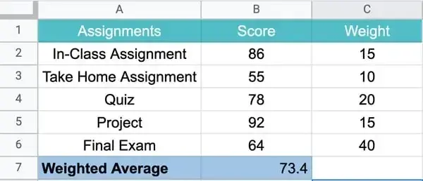
It then combines these values:

• 1290 + 550 + 1560 + 1380 + 2560 = 7340

Finally, the equation divides the combined value by the total value of our weights:

• 7340 / (15 + 10 + 20 + 15 + 40) = 73.4

How to find weighted moving averages in Excel

A useful variation of the weighted moving average is the weighted moving average.

When I use a weighted moving average, I can calculate an average over a period even as I add new data or give more weight to certain values. This can help identify trends and patterns more easily.

For example, if I know the number of views my website has received in the last five days, I can easily determine the average number of views over a five-day period.

Next week I want the same value, but from the last five days, not the five days from the previous week. This means I use the same time, but update the data to generate an average that takes the new data into account.

To find a weighted moving average, you give more weight to values ​​based on time.

In the example above, I’m assigning a weight to website views based on recency. More recent views (those that happened yesterday) are given more weight than those that happened five days ago. This means that every day I calculate using a moving average, the weights change.

Here’s what it looks like:

For the first set of five days I have 100, 200, 150, 300 and 100 views. I assign a weight to each of these days, with the last day having the most weight. To keep things simple, I’ll use weights that add up to 100.

• Day 1: 10 (x 100)
• Day 2: 15 (x 200)
• Day 3: 15 (x 150)
• Day 4: 25 (x 300)
• Day 5: 35 (x 100)

To get my weighted average, I use the formula from the previous section. I multiply each value by its weight and divide by the sum of the weights. For the specified values ​​we get: 172.5

On the sixth day, I restart the calculation of the weighted movement with new numbers. Our previous day 1 is no longer applicable — it has been replaced with values ​​from day 2, which is now our day 1. We also have a new data set from day 6 (total), which is now our day 5.

This means that the totals for days 2, 3, 4 and 5 are applied – they are just shifted one day to the left. Our new Day 5, meanwhile, has 200 views. Our weights say the same; all these changes are the number of views because they are related to the last five days.

Using our new data, our weighted moving average is calculated as follows:

• Day 1: 10 (x 200)
• Day 2: 15 (x 150)
• Day 3: 15 (x 300)
• Day 4: 25 (x 100)
• Day 5: 35 (x 200)

As a result, we get a new average, which is: 182.5

In Excel, you will need to manually enter this formula into each applicable cell.

WMA = [value 1 x (weight)] + [value 2 x (weight)] + [value 3 x (weight)] + [value 4 x (weight)] + [value 5 x (weight)] / total weight

Better than average: Mastering Excel operations

Once you get the hang of it, I think using the weighted average formula will become pretty easy. All it takes is a little practice. Although the weighted moving average is a bit more complicated, it is a great way to track performance data over time.

But that’s just the tip of Excel’s iceberg. With practice and a little help from our Excel hacks guide, you can master the art of equations. See below.

Editor’s note: This post was originally published in April 2022 and has been updated for comprehensiveness.